The Simulations Behind Comment 3

Last week I published what I submitted to the FDA on their January 2026 Bayesian guidance. Comment 3 argued that when you compose Bayesian trial components (priors, borrowing, sequential monitoring), the system's operating characteristics can diverge from what component-level analysis predicts. This post shows you the math.

The setup

Consider a single-arm trial with a binary endpoint, designed to detect an improvement in response rate over a historical null of 0.30 (based on 100 historical patients, 30 responders). The trial uses a dynamic mixture prior that borrows from historical data, with three sequential looks at n = 30, 60, and 90 patients.

The prior is a two-component mixture: an informative Beta(31, 71) derived from historical data and a weakly informative Beta(1, 1). At baseline, the informative component gets weight w₀ = 0.70. Dynamic borrowing updates that weight at each interim analysis, increasing it when accumulating data is consistent with the historical rate and decreasing it when there's conflict.

Success is declared when the posterior probability P(p > 0.30 | data) exceeds a threshold c, calibrated to control overall Type I error at 0.025 (one-sided).

There are two ways to calibrate this threshold. The composed approach simulates the full pipeline (dynamic weight updating interacting with sequential looks) and finds c = 0.963. The component approach fixes the prior weights at their starting values, runs the sequential design, and finds c = 0.961.

These differ by 0.002. But that's where the story starts, not where it ends.

All simulations below use conjugate Beta-Binomial computations. No MCMC, no external packages, no approximations. Fifty thousand replications per scenario. The R script runs in under three minutes.

Finding 1: The prior changes between looks

Under the null (true p = 0.30, matching the historical rate), the dynamic weight on the informative component doesn't stay at 0.70. It rises, to roughly 0.90 by the final look. Accumulating data that's consistent with the historical information strengthens the borrowing.

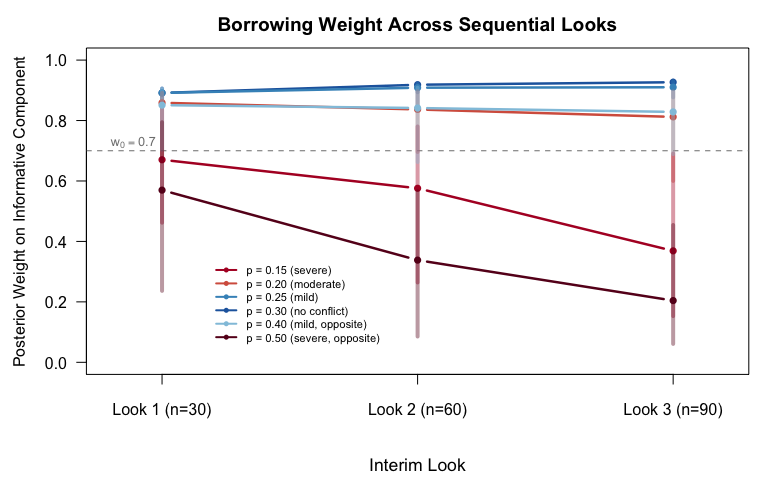
This matters because the sequential design evaluates a different prior at each look than the one it was calibrated against under a fixed-weight assumption. At Look 1 (n = 30), the effective prior is already more aggressive than the starting mixture. By Look 3 (n = 90), the trial is borrowing substantially more historical information than a component-level analysis would suggest.

Under drift, when the true response rate is lower than the historical rate, the picture reverses. The dynamic mechanism detects the conflict and collapses the informative weight, sometimes to near zero. But the collapse isn't instant. At early looks with limited data, the mechanism can't yet distinguish drift from noise, so borrowing persists longer than a sponsor might expect.

Finding 2: Effective sample size is bimodal under drift

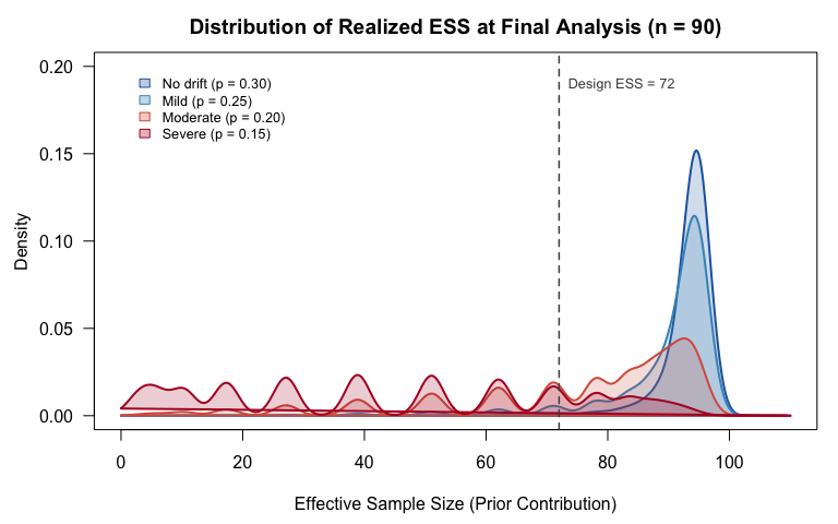
The trial was designed assuming an effective sample size (ESS) of 72 from the informative prior. Under the null, that's roughly correct: the weight increases, and realized ESS is higher than the starting assumption. Under severe drift (true p = 0.15 vs. historical 0.30), something more interesting happens.

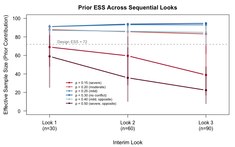
The ESS distribution at the final look is bimodal. In one mode, the dynamic mechanism detects the conflict and slashes borrowing, collapsing ESS to around 2. In the other mode, the data is ambiguous enough that the mechanism doesn't fully trigger, so ESS persists near 90. The design ESS of 72 sits in the gap between these modes where almost no simulations actually land.

Twenty-four percent of simulations under severe drift produce an ESS below 20. The sample size calculation assumed a stable ESS that, in practice, rarely occurs. No component-level ESS analysis, one that evaluates the prior in isolation from the sequential design, would reveal this bimodality.

Finding 3: A 0.002 threshold gap inflates Type I error by 33%

Here's the practical consequence. The component-calibrated threshold (c = 0.961) applied to the dynamic trial produces an overall Type I error of 0.020, versus the 0.015 that the composed calibration achieves. That's a 33% inflation in the error rate the sponsor would report to the agency.

The mechanism is concentrated at early looks. At Look 1 (n = 30), the dynamic design spends 0.0065 in alpha. The component calibration, which assumes fixed weights, would predict spending of 0.0006 at that look, an order of magnitude less. The more aggressive borrowing under the null makes early stopping more likely than a fixed-weight analysis suggests.

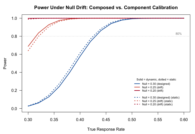
The power curves tell a complementary story. Under the design null (p = 0.30), the composed and component calibrations diverge modestly. Under drift, the gap widens further because the dynamic mechanism's behavior under the alternative also changes relative to what fixed-weight analysis predicts.

So what?

This is a toy example. Beta-Binomial with closed-form posteriors, a two-component mixture, three scheduled looks. Real submissions use MCMC for complex endpoints, adaptive randomization, time-to-event models with informative censoring, and multi-source external data. If composition effects are visible in the simplest case, they're likely worse in practice.

That's the substance of Comment 3's recommendation: Section VIII documentation in the guidance should require end-to-end simulation grids that evaluate the composed system, not just its parts. When the FDA reviews a Bayesian submission, the operating characteristics that matter are the ones that emerge from the pipeline the sponsor actually runs, not from a decomposition that may obscure interactions between components.

50,000 simulations · set.seed(20260307) · Base R, no external packages · R script