The Antidote to Guaranteed Significance

What to do instead of UPSIs

On December 22, 2025, Dr. Hackman published a guide to guaranteeing significant results. If cheating at science is your goal, he says, it’s required reading.

I spent nearly a decade writing SAPs designed to prevent exactly this. The 92% false positive rate he demonstrated isn’t surprising—it’s the reason regulatory statisticians exist.

His post ends with a promise: future threads on what to do instead. I got impatient.

This is the antidote.

The setup

Hackman’s simulation uses 6 covariates to define subgroups:

library(tidyverse)
library(broom)

set.seed(21)
n <- 100

subgroups <- expand.grid(
  age = c("18-35", "36-50", "51-65", "66-80", "80+"),
  sex = c("Male", "Female"),
  hand = c("Left", "Right"),
  coffee = c("0", "1", "2+"),
  alcohol = c("0", "1", "2", "3+"),
  physical_activity = c("0", "1", "2", "3+")
)

That’s 960 possible subgroups. With pairwise interactions in the model matrix, you’re searching through ~93 candidate predictors. Then you run forward stepwise selection with BIC, report the p-values as if model selection never happened, and publish.

The result: false positives in 92% of simulations, from pure noise.

The simplest fix: multiplicity corrections

I’ve reviewed protocols where the analysis plan specified dozens of subgroup comparisons with no adjustment. When I flagged multiplicity, the response was usually some version of “but we’re using BIC for selection, so it’s principled.”

It’s not. Selection doesn’t make the multiple testing problem disappear. It makes it harder to see.

The simplest antidote: adjust the p-values for the number of tests you ran, or could have run.

simulate_with_corrections <- function(seed = NULL) {
  if (!is.null(seed)) set.seed(seed)
  
  y <- rnorm(n)
  x_idx <- sample(1:nrow(subgroups), n, replace = TRUE)
  X <- subgroups[x_idx, ]
  simdata <- data.frame(y = y, X)
  X2 <- model.matrix(y ~ . * ., data = simdata)[, -1]
  simdata2 <- data.frame(y = y, X2)
  
  null_model <- lm(y ~ 1, data = simdata2)
  full_model <- lm(y ~ ., data = simdata2)
  
  selected <- step(null_model,
                   scope = list(lower = null_model, upper = full_model),
                   direction = "forward",
                   k = log(n),
                   trace = 0)
  
  coefs <- tidy(selected) |> filter(term != "(Intercept)")
  
  if (nrow(coefs) == 0) {
    return(tibble(
      method = c("Unadjusted", "Bonferroni", "Holm", "BH (FDR)"),
      any_sig = FALSE
    ))
  }
  
  p_raw <- coefs$p.value
  n_candidates <- ncol(X2)
  
  tibble(
    method = c("Unadjusted", "Bonferroni", "Holm", "BH (FDR)"),
    any_sig = c(
      any(p_raw < 0.05),
      any(pmin(p_raw * n_candidates, 1) < 0.05),
      any(p.adjust(p_raw, method = "holm", n = n_candidates) < 0.05),
      any(p.adjust(p_raw, method = "BH", n = n_candidates) < 0.05)
    )
  )
}

corrected_results <- map(1:50, ~simulate_with_corrections(seed = .x))

corrected_summary <- bind_rows(corrected_results) |>
  group_by(method) |>
  summarize(pct_sig = mean(any_sig) * 100, .groups = "drop") |>
  mutate(method = factor(method, levels = c("Unadjusted", "Bonferroni", "Holm", "BH (FDR)")))

ggplot(corrected_summary, aes(x = method, y = pct_sig, fill = method)) +
  geom_col(width = 0.7) +
  geom_hline(yintercept = 5, linetype = "dashed", color = "#472d30", linewidth = 1) +
  annotate("text", x = 4.2, y = 8, label = "Nominal α = 5%", color = "#472d30", size = 3.5) +
  scale_fill_manual(values = c("#723d46", "#e26d5c", "#ffe1a8", "#c9cba3")) +
  labs(x = NULL, y = "% of simulations with ≥1 'significant' result") +
  theme_minimal(base_size = 13) +
  theme(legend.position = "none")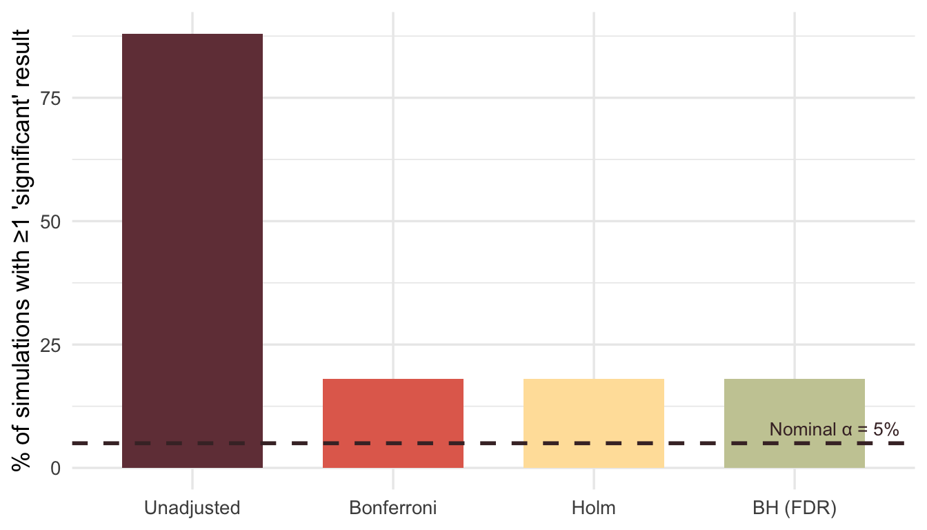

Even Bonferroni—blunt as it is—brings the false positive rate back to earth.

A caveat: adjusting p-values after selection is better than nothing, but it’s not ideal. The proper adjustment depends on the selection procedure itself. Packages like selectiveInference attempt to do this correctly, but the methods are complex and often conservative. In practice, the bigger win is not relying on post-hoc selection in the first place.

It’s worse than you think

Hackman’s example is a toy. Six covariates. A hundred patients. Real trials are messier.

I’ve worked on oncology protocols with subgroup definitions like this:

onc_subgroups <- expand.grid(
  age = c("<65", "≥65"),
  sex = c("Male", "Female"),
  ecog = c("0", "1", "2+"),
  prior_lines = c("0", "1", "2+"),
  biomarker = c("Positive", "Negative", "Unknown"),
  stage = c("III", "IV"),
  histology = c("Adeno", "Squamous", "Other"),
  region = c("North America", "Europe", "Asia", "ROW")
)

That’s 2,592 subgroups from 8 variables. And this is still simplified. Real protocols track tumor mutation burden, PD-L1 expression levels, specific genetic alterations, smoking history, CNS involvement, liver metastases, LDH levels. I’ve seen subgroup tables in SAPs run for pages.

The combinatorics get absurd fast. This is why regulatory statisticians are paranoid about multiplicity. It’s not pedantry—it’s the only thing standing between a promising subgroup signal and a failed Phase 3.

The Bayesian alternative

Rather than testing each subgroup independently, Bayesian hierarchical models treat subgroup effects as drawn from a common distribution. Extreme estimates get pulled toward the overall mean—shrinkage—reflecting the prior belief that subgroups probably aren’t wildly different from each other.

library(rstanarm)

set.seed(42)
n_per_group <- 20
groups <- LETTERS[1:10]

bayes_demo <- tibble(
  group = rep(groups, each = n_per_group),
  y = rnorm(n_per_group * length(groups))  # No true effect
)

# Frequentist: separate estimate per group
freq_fit <- lm(y ~ group - 1, data = bayes_demo)
freq_est <- tidy(freq_fit) |>
  transmute(group = str_remove(term, "group"), estimate, method = "No Pooling")

# Bayesian hierarchical model
bayes_fit <- stan_lmer(
  y ~ (1 | group),
  data = bayes_demo,
  prior_intercept = normal(0, 1),
  seed = 123,
  refresh = 0
)

bayes_est <- as_tibble(ranef(bayes_fit)$group, rownames = "group") |>
  transmute(
    group,
    estimate = `(Intercept)` + fixef(bayes_fit)["(Intercept)"],
    method = "Partial Pooling"
  )

comparison <- bind_rows(freq_est, bayes_est)

ggplot(comparison, aes(x = group, y = estimate, color = method, shape = method)) +
  geom_hline(yintercept = 0, linetype = "dashed", color = "gray50") +
  geom_point(size = 3.5, position = position_dodge(width = 0.4)) +
  scale_color_manual(values = c("No Pooling" = "#ee6c4d", "Partial Pooling" = "#3d5a80")) +
  labs(x = "Subgroup", y = "Estimated Effect", color = NULL, shape = NULL) +
  theme_minimal(base_size = 13) +
  theme(legend.position = "bottom")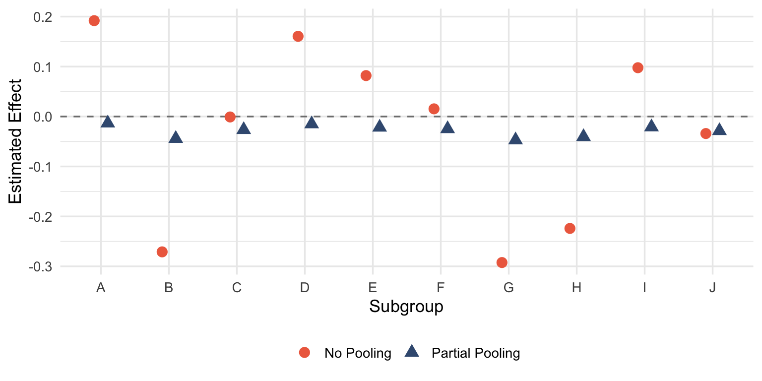

The red points scatter wildly around zero—each group estimated in isolation, free to wander wherever the noise takes it. The blue points huddle closer to the grand mean. When there’s no true effect, that’s exactly what you want.

This isn’t magic. The model is encoding a reasonable assumption: subgroups are more similar than different until proven otherwise. If a subgroup really is exceptional, the data will overcome the prior. If it’s not, the estimate gets regularized back toward the population effect.

Pre-specified hierarchical testing

This is what FDA expects. You declare your testing strategy before unblinding:

1. Test the primary endpoint at α = 0.05
2. Only if the primary is significant, test the key secondary at α = 0.05
3. Only if the key secondary is significant, test pre-specified subgroups

The alpha doesn’t pass down unless each gate opens.

simulate_hierarchical <- function(seed = NULL) {
  if (!is.null(seed)) set.seed(seed)
  
  n_trial <- 200
  dat <- tibble(
    y = rnorm(n_trial),
    trt = rep(c(0, 1), each = n_trial/2),
    biomarker = sample(c("pos", "neg"), n_trial, replace = TRUE),
    age_group = sample(c("young", "old"), n_trial, replace = TRUE)
  )
  
  # Gate 1: Primary
  p_primary <- tidy(lm(y ~ trt, data = dat))$p.value[2]
  gate1 <- p_primary < 0.05
  
  # Gate 2: Key secondary (only if gate 1 passed)
  p_secondary <- tidy(lm(y ~ trt, data = filter(dat, biomarker == "pos")))$p.value[2]
  gate2 <- gate1 && (p_secondary < 0.05)
  
  # Gate 3: Exploratory
  p_exploratory <- tidy(lm(y ~ trt, data = filter(dat, age_group == "young")))$p.value[2]
  gate3 <- gate2 && (p_exploratory < 0.05)
  
  c(primary = gate1, secondary = gate2, exploratory = gate3)
}

hier_results <- map(1:500, ~simulate_hierarchical(seed = .x))
hier_rates <- colMeans(do.call(rbind, hier_results)) * 100

Over 500 null simulations:

• Primary endpoint “significant”: 5%
• Key secondary claimed: 1.4%
• Exploratory subgroup claimed: 0.8%

The family-wise error rate stays controlled because downstream claims require upstream significance first. It’s not elegant, but it works.

The real antidote

The methods above help, but they’re all downstream fixes. The actual solution is boring: decide what you’re testing before you see the data. Write it in the SAP. Register it. Then do what you said you’d do.

Hackman’s approach works because it exploits the gap between what researchers could test and what they claim to have tested. Pre-specification closes that gap. Not perfectly—there’s still analyst degrees of freedom, still judgment calls in implementation—but enough to make the 92% false positive rate impossible.

The dark arts work because we let them. In clinical trials, where patients’ lives depend on honest inference, we don’t have that luxury.

This post is a response to How can I guarantee a significant result? by Perry Hackman at Data Diction.