In Defense of 50:50 Randomization

I’ve been in meetings where “adaptive” was treated as a synonym for “smaller trial.”

The assumption goes like this: if we can learn as we go, we can stop early when something works, drop arms that fail, and route patients to better treatments. Surely that means fewer patients overall.

The math says otherwise.

BATTLE, the trial I praised last month for doing adaptive randomization right, was estimated to be 74% larger than a fixed design with interim monitoring would have been. Not smaller. Larger.

This isn’t a BATTLE problem. It’s a category error about what adaptive designs actually optimize for.

The misconception

The pitch usually sounds like this:

“With adaptive randomization, we assign more patients to the better arm as we learn. We’ll need fewer patients to detect a difference, and more of them will benefit.”

Both claims are wrong.

Why 50:50 is always more efficient

This is textbook, but it surprises people: balanced randomization maximizes statistical efficiency for estimating treatment effects.

The variance of a treatment effect estimate depends on sample size in each arm. For a two-arm trial with total sample size $N$, the variance of the difference in means is minimized when $n_1 = n_2 = N/2$.

library(tidyverse)

# Variance of difference in means as function of allocation
# Var(Y1_bar - Y2_bar) = sigma^2 * (1/n1 + 1/n2)
# With N total and proportion p to arm 1:
# Var = sigma^2 * (1/(pN) + 1/((1-p)N)) = sigma^2/N * (1/p + 1/(1-p))

allocation_variance <- tibble(
  p = seq(0.1, 0.9, by = 0.01),
  relative_variance = (1/p + 1/(1-p)) / 4  
  # Normalized so 50:50 = 1
)

ggplot(allocation_variance, aes(x = p, y = relative_variance)) +
  geom_line(linewidth = 1, color = "#3d5a80") +
  geom_point(data = tibble(p = 0.5, relative_variance = 1), 
             size = 3, color = "#ee6c4d") +
  geom_hline(yintercept = 1, linetype = "dashed", color = "gray50") +
  annotate("text", x = 0.42, y = 1.12, label = "50:50 allocation", 
           hjust = 0, color = "#ee6c4d") +
  scale_x_continuous(labels = scales::percent) +
  labs(
    x = "Proportion Allocated to Arm 1",
    y = "Relative Variance (vs. 50:50)",
    title = "Unequal allocation always costs you precision"
  ) +
  theme_minimal(base_size = 13)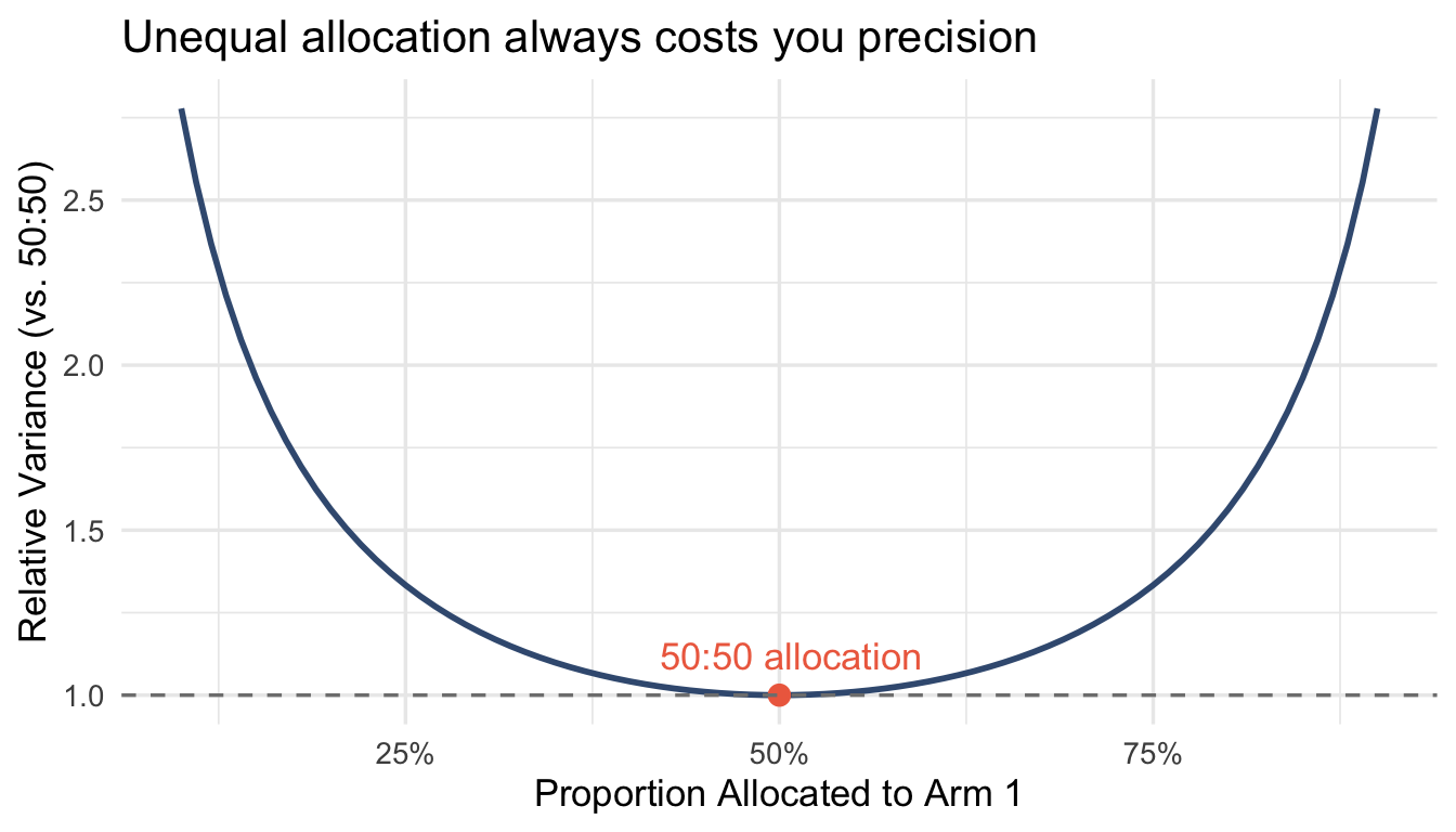

At 70:30 allocation, you need ~17% more patients to achieve the same precision as 50:50. At 80:20, it’s 56% more.

Response-adaptive randomization deliberately moves away from 50:50. That’s the point—route patients to better treatments. But the cost is statistical efficiency. You’re trading estimation precision for within-trial patient benefit.

That trade might be worth it. But it’s not free, and it doesn’t save you sample size.

The wrong-direction problem

It gets worse. Adaptive randomization doesn’t reliably send more patients to the better arm—especially early in a trial when estimates are noisy.

A simple simulation illustrates the mechanics. With a true 15-percentage-point treatment benefit and 200 patients, my Thompson Sampling implementation sends more patients to the better arm about 94% of the time. Sounds good.

But this is a favorable scenario: large effect, moderate sample size, fast outcomes. Thall’s more rigorous simulations in Annals of Oncology tell a different story. Under realistic conditions—smaller effects, slower accrual, noisier endpoints—Thompson Sampling produces 14% to 43% probability of allocating more patients to the inferior arm.

That’s not a rounding error. That’s one in three trials sending more patients to the worse treatment while claiming ethical superiority.

The “more patients get the better treatment” justification assumes the adaptation works as intended. When it doesn’t—and it frequently doesn’t—you’ve traded statistical efficiency for nothing.

The BATTLE numbers

Korn and Freidlin analyzed BATTLE in the Journal of the National Cancer Institute. Their estimate: the adaptive design was 74% larger than a fixed-randomization design with equivalent interim monitoring would have been.

Translated: BATTLE potentially exposed 65% more patients to treatment failure than a simpler design.

This wasn’t because BATTLE was poorly designed. It was because the trial optimized for something other than sample size—namely, learning about biomarker-treatment interactions in real time. That’s a legitimate objective. But it’s not efficiency.

When does adaptation actually save patients?

Early stopping for efficacy or futility—via group sequential designs—genuinely saves patients. The key: you stop the whole trial, not just shift allocation.

# Compare fixed vs group sequential under various effect sizes
# Using manual O'Brien-Fleming boundaries to avoid rpact complexity

# Design parameters
alpha <- 0.025
power <- 0.90
effect_assumed <- 0.3
sigma <- 1

# Fixed design sample size (per arm)
n_per_arm_fixed <- ceiling(2 * ((qnorm(1 - alpha) + qnorm(power)) * sigma / effect_assumed)^2)
n_fixed <- n_per_arm_fixed * 2

# O'Brien-Fleming approximate boundaries for 3 looks at 33%, 67%, 100%
# These are standard values
of_boundaries <- c(3.471, 2.454, 2.004)
info_rates <- c(0.33, 0.67, 1.0)

# GSD max sample size (inflated ~3% for 3 looks with OF)
n_gsd_max <- ceiling(n_fixed * 1.03)
n_per_arm_gsd <- ceiling(n_gsd_max / 2)

# Simulate expected sample size under different true effects
simulate_gsd_expected_n <- function(true_effect, n_sims = 2000) {
  
  stopped_n <- numeric(n_sims)
  
  for (i in 1:n_sims) {
    # Generate full dataset
    y_control <- rnorm(n_per_arm_gsd, 0, sigma)
    y_treatment <- rnorm(n_per_arm_gsd, true_effect, sigma)
    
    stopped <- FALSE
    
    for (j in seq_along(info_rates)) {
      n_look <- max(5, floor(n_per_arm_gsd * info_rates[j]))
      
      # Two-sample z-test
      mean_diff <- mean(y_treatment[1:n_look]) - mean(y_control[1:n_look])
      se <- sigma * sqrt(2 / n_look)
      z_stat <- mean_diff / se
      
      # Check efficacy boundary
      if (!is.na(z_stat) && z_stat > of_boundaries[j]) {
        stopped_n[i] <- n_look * 2
        stopped <- TRUE
        break
      }
    }
    
    if (!stopped) {
      stopped_n[i] <- n_gsd_max
    }
  }
  
  mean(stopped_n)
}

effects <- seq(0, 0.5, by = 0.05)
expected_n <- map_dbl(effects, simulate_gsd_expected_n)

gsd_comparison <- tibble(
  true_effect = effects,
  fixed = n_fixed,
  gsd_expected = expected_n,
  savings_pct = (n_fixed - expected_n) / n_fixed * 100
)

gsd_comparison |>
  select(true_effect, fixed, gsd_expected) |>
  pivot_longer(-true_effect, names_to = "design", values_to = "n") |>
  mutate(design = ifelse(design == "fixed", "Fixed", "Group Sequential (expected)")) |>
  ggplot(aes(x = true_effect, y = n, color = design, linetype = design)) +
  geom_line(linewidth = 1) +
  geom_vline(xintercept = 0.3, linetype = "dotted", color = "gray40") +
  annotate("text", x = 0.305, y = max(gsd_comparison$fixed) * 0.975, 
           label = "Design Assumption", hjust = 0, size = 3, color = "gray25") +
  scale_color_manual(values = c("Fixed" = "#ee6c4d", "Group Sequential (expected)" = "#3d5a80")) +
  labs(
    x = "True Effect Size",
    y = "Sample Size",
    color = NULL, linetype = NULL,
    title = "Group sequential designs save patients when effects are large"
  ) +
  theme_minimal(base_size = 13) +
  theme(legend.position = "bottom")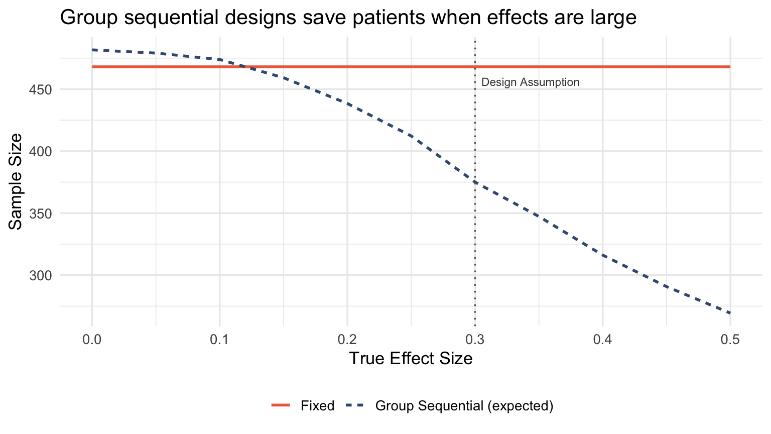

When the true effect is larger than expected, group sequential designs stop early and save substantial sample size. When the effect matches the design assumption, the expected sample size is close to fixed. When the effect is smaller (or null), you pay a modest inflation for the interim looks.

This is genuine efficiency—not reallocation theater.

The follow-up problem

Adaptive randomization requires fast outcomes. If your endpoint takes 12 months and you enroll 20 patients per month, you’ll randomize 240 patients before seeing a single outcome. The “adaptation” is decorative.

# Visualize the follow-up to enrollment ratio problem

followup_scenarios <- tibble(
  scenario = c(
    "8-week DCR\n(BATTLE)",
    "6-month PFS",
    "12-month OS",
    "24-month OS"
  ),
  followup_months = c(2, 6, 12, 24),
  enrollment_rate = 20  # patients per month
)

followup_scenarios <- followup_scenarios |>
  mutate(
    patients_before_first_outcome = followup_months * enrollment_rate,
    scenario = factor(scenario, levels = scenario),
    can_adapt = followup_months <= 3
  )

ggplot(followup_scenarios, aes(x = scenario, y = patients_before_first_outcome, fill = can_adapt)) +
  geom_col(width = 0.6) +
  geom_hline(yintercept = 100, linetype = "dashed", color = "gray40") +
  annotate("text", x = 4.33, y = 120, label = "Typical Phase II size", 
           hjust = 1, size = 3, color = "gray25") +
  scale_fill_manual(values = c("TRUE" = "#3d5a80", "FALSE" = "#ee6c4d"), guide = "none") +
  labs(
    x = NULL,
    y = "Patients enrolled before first outcome observed",
    title = "Slow endpoints make adaptive randomization pointless",
    subtitle = "Assumes 20 patients/month enrollment"
  ) +
  theme_minimal(base_size = 13)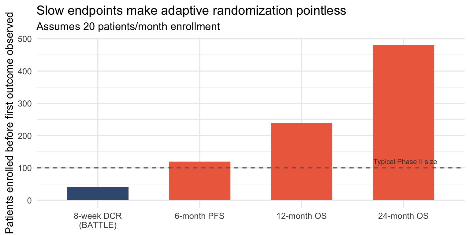

BATTLE worked because the endpoint was 8-week disease control. By the time 40 patients were enrolled, 8-week data from the first cohort was available. The adaptation could actually happen.

For trials powered on overall survival, adaptive randomization is usually fiction.

When to actually use adaptive designs

Adaptive randomization makes sense when:

• Routing is the objective — platform trials where assigning patients to promising arms is itself the scientific goal
• Outcomes are fast — weeks, not months
• Multiple arms are competing — the efficiency loss per comparison is offset by dropping losers
• Within-trial patient benefit matters more than estimation precision — rare disease, no other options

It doesn’t make sense when:

• You need precise treatment effect estimates — balanced allocation wins
• Endpoints are slow — you’ll finish before adapting
• Regulatory confirmation is the goal — FDA still prefers group sequential
• You’re calling it adaptive but constraining it to irrelevance

The takeaway

Adaptive designs don’t mean smaller trials. They mean different trials—optimized for different objectives, with different trade-offs.

The efficiency gains come from stopping early, not from reallocating patients. Group sequential designs have been doing this for decades without the operational complexity.

Next time someone pitches an adaptive design as a sample size discount, ask two questions:

1. What’s the follow-up to enrollment ratio?
2. Show me the simulation where RAR beats group sequential on expected sample size.

The answers will be revealing.

This post follows up on What BATTLE Got Right That Most Adaptive Trials Get Wrong, which explored when adaptive randomization actually works.

📬 Want more insights? Subscribe to the newsletter or explore the full archive of Evidence in the Wild for more deep dives into experimental design.