Bayesian Priors in Clinical Trials: Why Historical Borrowing Reduces Sample Size
A post circulating on LinkedIn last week made a familiar claim: the only difference between Bayesian and frequentist statistics is the prior, and with an uninformative prior the two frameworks give identical answers. The author ran simulations with a Beta(1,1) prior to prove it.
That statement is mathematically correct. With a flat prior, Bayesian posterior inference and frequentist likelihood inference converge. But the conclusion often drawn from it (that priors are therefore a minor implementation detail) is exactly backwards.
The interesting question isn't what happens when you make the prior as weak as possible. It's what happens when you make it as informative as the evidence justifies. And the answer to that question has direct consequences for how many patients you need to enroll in a trial.
The setup
Consider a standard binary endpoint trial: control arm response rate of 20%, treatment arm of 35%, and a decision rule based on the posterior probability that treatment beats control. This is not a contrived scenario: it maps directly onto the kind of oncology trials I spent years designing.
Now suppose you have historical control data. Maybe you ran an identical control arm in a prior trial. Maybe there's a well-characterized natural history cohort. You have information about the control rate that predates your current study. The Bayesian approach lets you encode that information as a prior on the control arm.
The question is: compared to a design that ignores that historical data, how much does borrowing it cost you in sample size to reach the same power at the same Type I error?
The short answer from the simulation: a lot.
What the simulation shows
I ran 2,000 simulated trials for each combination of prior and sample size, using an analytical computation of P(treatment > control) to avoid Monte Carlo noise in the inner loop. Critically, every design is calibrated to hold Type I error at 5% before comparing power; the power differences are real, not an artifact of uncalibrated thresholds.
Three control-arm priors, all centered at the true control rate of 20%, varying only in how much historical data they encode:
| Prior | ESS | Interpretation |
|---|---|---|
| Beta(1,4) | ~5 | Minimal borrowing |
| Beta(4,16) | ~20 | ~20 historical patients |
| Beta(10,40) | ~50 | ~50 historical patients |
In a Beta–Binomial model, the effective sample size of a Beta(a,b) prior is often interpreted as a+b pseudo-observations. This is not a literal dataset; it is a convenient scale for quantifying how much historical information the prior contributes relative to the trial data.
Figure 1 shows calibrated power curves across a range of per-arm sample sizes.
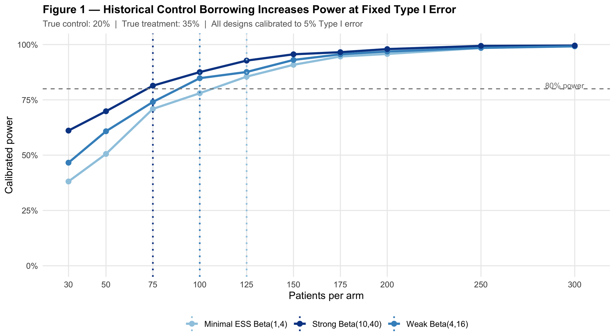
The strong prior (ESS = 50) reaches 80% power at N = 75 patients per arm. The minimal-ESS prior needs N = 125 patients per arm for the same target. That's 100 fewer patients randomized, all from encoding roughly 50 patients of historical control data at the correct rate.
This is not a statistical trick. The thresholds are different: the stronger prior reaches its decision threshold with less trial data because it arrived at the analysis with more information already in hand. The Type I error is held fixed at 5% for all three designs throughout. The power gain is a direct consequence of the additional information encoded in the prior ESS.
What happens when the historical data is wrong
This is where the analysis gets interesting, and where most LinkedIn-friendly Bayesian explainers stop short.
Suppose the historical control rate wasn't 20%. Maybe it was 30% (a pessimistic prior: you overestimate how well the control arm performs). Maybe it was 8% (an optimistic prior: you underestimate it). You encode that misinformation into your prior with the same ESS of 50, calibrate your threshold under each scenario's own null, and ask what happens.
Figure 2 shows calibrated power and empirical Type I error under each misspecification scenario.
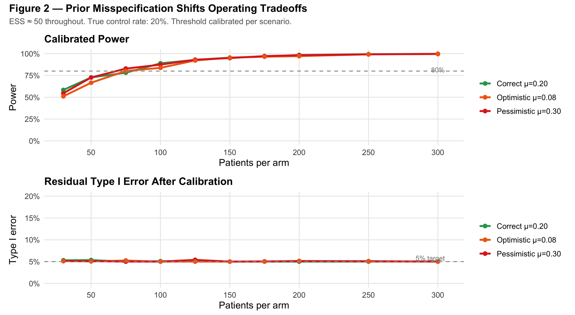
The story here is not symmetric, but it's also not catastrophic, and the distinction matters for how you interpret it.
Because calibration is done per-scenario, calibration largely absorbs the Type I error distortion that prior misspecification would otherwise introduce. The more consequential operating differences show up in the calibrated threshold and in power:
- Pessimistic prior (overestimates control at 30%): conservative. The design requires a lower decision threshold to hit 5% Type I error, and power drops meaningfully as a result. You're leaving power on the table.
- Optimistic prior (underestimates control at 8%): requires a stricter calibrated threshold and is more sensitive to prior–data conflict. Under real-world drift between historical and current controls (which is the actual risk in practice), and that lack of robustness becomes more consequential.
The practical implication: in this setup, the direction of prior misspecification matters more than its magnitude, and an optimistic prior carries more tail risk than a pessimistic one. If you're uncertain about which way your historical data might be biased, conservative misspecification is the safer error.
The self-correcting property
The natural objection to all of this is: what if the prior is badly wrong and I'm stuck with it? This is where Bayesian inference has a structural advantage that's worth making concrete.
Figure 3 shows posterior mean trajectories for the control arm across 500 simulated datasets, with 50% and 95% empirical quantile bands. All three priors (correct, pessimistic, and optimistic) have the same ESS of ~50.
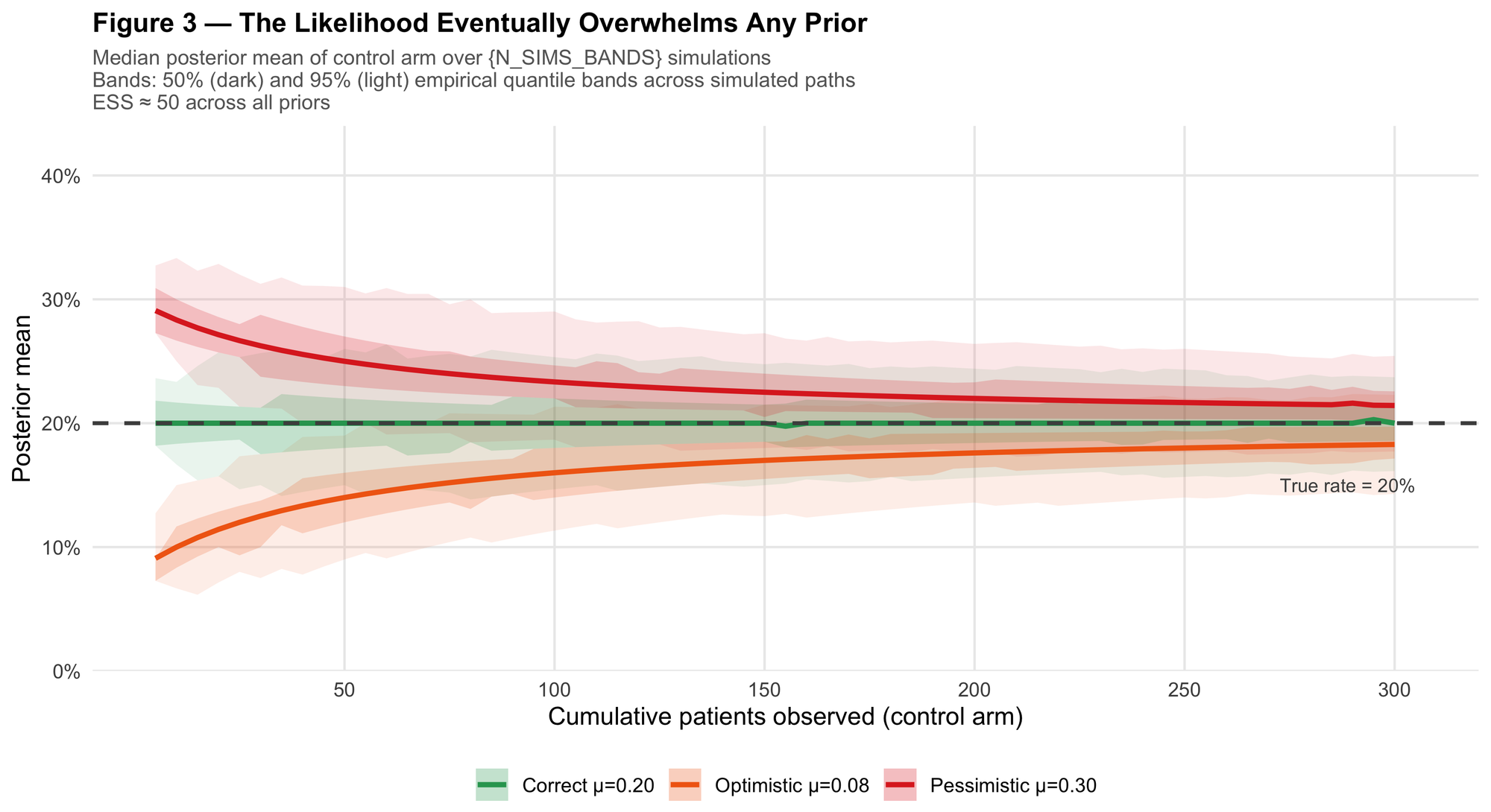
The pessimistic prior starts high (near 30%). The optimistic prior starts low (near 8%). Both median trajectories approach the true 20% rate roughly in the N = 100–150 range. With enough accumulating data, the likelihood pulls the posterior toward the truth even when the prior is misspecified.
This is not a guarantee: it's a property that holds in large enough samples, for the priors and sample sizes studied here. But it is a meaningful reassurance: a well-designed trial doesn't depend on the prior being exactly right. It depends on the prior being reasonable, and the data being sufficient to correct it if it isn't.
Why this connects to FDA's January 2026 guidance
FDA's Bayesian guidance, released in January 2026, addresses historical control borrowing directly. The framework it endorses isn't "use flat priors to mimic frequentist analysis." It's a principled approach to encoding prior information at a pre-specified level of borrowing, evaluating operating characteristics under prior–data conflict scenarios, and calibrating decision thresholds to frequentist targets.
In practice, historical control borrowing is often implemented through frameworks such as power priors, commensurate priors, or meta-analytic predictive (MAP) priors, all designed to modulate how strongly historical data influence the current analysis. The simulation here uses a simple conjugate Beta prior to keep the mechanics transparent, but the operating logic is the same across all three approaches.
This simulation mirrors the framework the guidance expects: prespecify the borrowing, calibrate the decision rule to frequentist operating characteristics, and evaluate robustness under plausible prior–data conflict scenarios. Regulators want to see all three, and the simulation structure here maps cleanly onto that checklist.
The bottom line
The LinkedIn post that prompted this analysis was making a narrow mathematical point: flat priors give flat posteriors that agree with the likelihood. Fine. But if your historical data is good enough to encode a prior with ESS = 50, using a flat prior instead is equivalent to throwing away 50 patients of information. In a 150-patient trial, that's a third of your evidence base.
Informative priors on the control arm aren't a way to cheat the data. They're a mechanism for putting existing knowledge to work, at a controlled, calibrated Type I error rate. The sample size savings are real, the risks of misspecification are quantifiable and manageable, and the data will eventually correct even a badly specified prior.
The prior isn't the problem. For many trials with credible historical data, the real question is whether you can justify ignoring one.
The full simulation code is available as a Quarto document. All figures are reproducible with the published seed.
If you're staring at a historical control dataset and trying to decide how much to borrow, that's exactly the kind of problem I work on with sponsors. I do independent consulting on Bayesian trial design, simulation-based calibration, and FDA-facing analysis plans. More at evidenceinthewild.com/services.
Member discussion